Individual Science Windows Spectra

Let us first proceed with the spectral extraction using the source positions found at the IMA step. In our example only the Crab was found by the imaging analysis, so the spectral analysis will generate only the spectrum of the Crab if you run the script with default values (assuming you run j_rebin_rmf in your $REP_BASE_PROD directory):

cd $REP_BASE_PROD/obs/crab

jemx_science_analysis startLevel="SPE" endLevel="SPE" jemxNum=2\
   response="$REP_BASE_PROD/jemx_rebinned_rmf.fits"

The results of the spectral analysis data are in the file

scw/RRRRPPPPSSSF.001/jmx2_srcl_spe.fits

Look on the result of the spectral analysis of the Science Window 010200210010

cd scw/010200210010.001/
fv jmx2_srcl_spe.fits

In this file you find the spectra for all sources that were found at the IMA level. Note that the correspondence between source name and source ID can be found in the file jmx2_srcl_res.fits.

Figure 18: Left panel: Crab spectrum in ScW 010200210010. Right panel: Combined Crab spectrum of ScW 010200210010 and ScW 010200220010.

The JEM-X systematics are of the order of a few percents, typically 3%. We add this explicitly to jmx2_srcl_spe.fits file with the command below:

fparkey 0.03 jmx2_srcl_spe.fits SYS_ERR add=yes

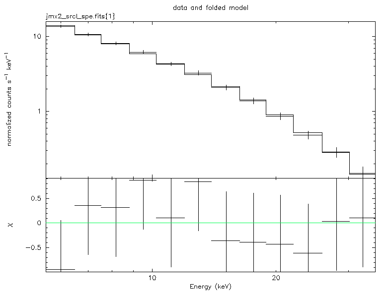
The obtained spectrum can be analysed e.g. within XSPEC program:

xspec
XSPEC>cpd /xw
XSPEC>data jmx2_srcl_spe.fits{1}
XSPEC>ign **-5.0
XSPEC>setplot energy
XSPEC>model po
XSPEC>fit
XSPEC>plot ldat del

The above set of XSPEC commands reads the data file and fits the data with ``power-law'' model. The result is shown in the left panel of Fig. 18. The fit results in a photon index of , and a normalisation at 1 keV of .

To understand the importance of the ``user catalog'' let us extract the Crab spectrum using the catalog position of the source, not the one found at the IMA level. For this you have to re-run the analysis starting from the very beginning, but specifying that you want to use your own catalog for the spectral and lightcurve extraction. Create a new observation group crab_usrcat

cd $REP_BASE_PROD
og_create idxSwg=jmx.lst ogid=crab_usrcat baseDir="./" instrument=JMX2

copy the user catalog created as explained above into the observation group

cp user_cat.fits obs/crab_usrcat

and run the analysis till SPE level in this group:

cd obs/crab_usrcat
jemx_science_analysis startLevel="COR" \
   endLevel="SPE" jemxNum=2 CAT_I_usrCat="user_cat.fits" \
   nChanBins=-4 response="$REP_BASE_PROD/jemx_rebinned_rmf.fits"

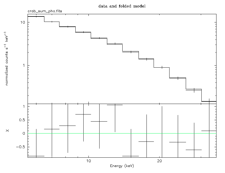
The obtained spectra can be analysed with XSPEC as it was done above. To convince yourself that the spectral extraction with and without fixing the source position gives slightly different results, you can compare the two spectra, $REP_BASE_PROD/obs/crab/scw/010200210010.001/jmx2_srcl_spe.fits and
$REP_BASE_PROD/obs/crab_usrcat/scw/010200210010.001/jmx2_srcl_spe.fits by entering them simultaneously in XSPEC.

With this OSA release, and until the flux determination algorithm in j_ima_iros is duplicated in a dedicated spectral extraction tool, it is not possible anymore to generate several spectra in a single analysis with a given time step. The user must define her/his own GTIs for the specific time period.