Spectral Extraction

Before starting, you may want to save your imaging analysis again, by copying the current directory

cd ..
cp -r spi_analysis  spi_imaging_with_catalogue
cd  spi_analysis

Spiros program can only extract spectra at fixed, known positions. Therefore, a source_cat.fits file must be provided in any case. We assume that you have created/checked a source_cat.fits as explained in last section. Launch ``spi_science_analysis'', un-select the catalogue extraction step, and provide the input catalogue name source_cat.fits in the ``spiros input catalogue'' field.

It is not necessary to run the pointing step again. However, the number of considered energy bins is typically much larger in spectral extractions than in imaging reconstructions. Select the binning, background, and spiros steps. In the energy binning step, you can now select a binning suitable for a spectrum of a bright source with a broader energy range and a relatively high number of bins. For our example, set the number of regions to "1", a "20,1000" keV boundary, and " " as the number of bins. As stated before, using a negative bin number implies a logarithmic binning, with 100 bins from 20keV up to 1MeV in our case.

Open the spiros GUI and set spiros mode to spectra instead of imaging. Click ``Ok'' and ``Run'' the pipeline. After spiros has finished successfully, the pipeline will automatically generate the appropriate response matrix and attach it to your spectra.

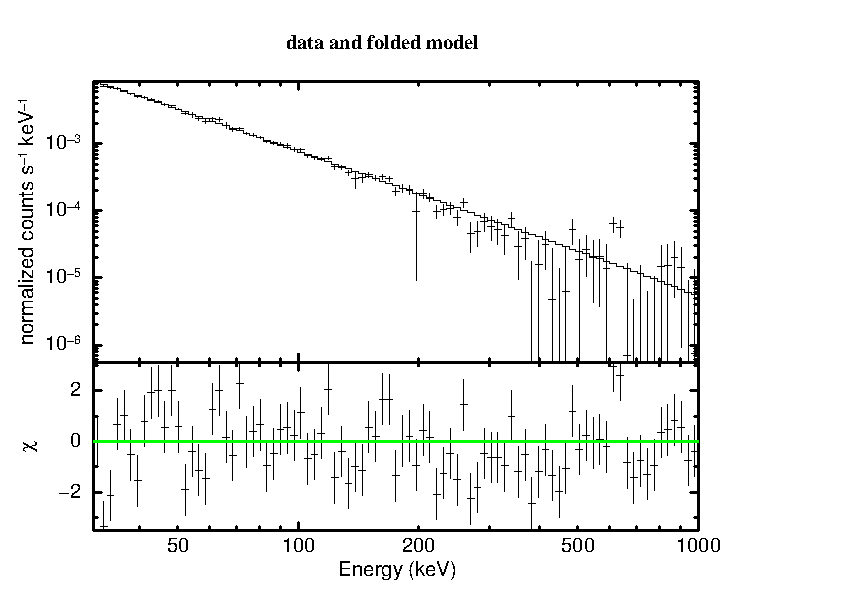
To evaluate the obtained results, you can use XSPEC to analyze your spectra. In the following example we fit a single power law from 30 to 1000keV. Here is a verbatim of the XSPEC session.

================================================================================
              XSPEC version: 12.8.2
    Build Date/Time: Tue Oct 21 17:05:03 2014
XSPEC12>data spectrum_Crab.fits

Spectral Data File: spectrum_Crab.fits  Spectrum 1
Net count rate (cts/s) for Spectrum:1  3.912e-01 +/- 3.232e-03
 Assigned to Data Group 1 and Plot Group 1
  Noticed Channels:  1-100
  Telescope: INTEGRAL Instrument: SPI  Channel Type: PI
  Exposure Time: 1.902e+04 sec
 Using fit statistic: chi
 Using test statistic: chi
 Using Response (RMF) File            spectral_response.rmf.fits for Source 1

XSPEC12>cpd /xw
XSPEC12>ign **-30.
    11 channels (1-11) ignored in spectrum #     1
XSPEC12>setpl en
XSPEC12>plot lda
XSPEC12>model power

Input parameter value, delta, min, bot, top, and max values for ...
              1       0.01(      0.01)         -3         -2          9         10
1:powerlaw:PhoIndex>
              1       0.01(      0.01)          0          0      1e+20      1e+24
2:powerlaw:norm>

========================================================================
Model powerlaw<1> Source No.: 1   Active/On
Model Model Component  Parameter  Unit     Value
 par  comp
   1    1   powerlaw   PhoIndex            1.00000      +/-  0.0
   2    1   powerlaw   norm                1.00000      +/-  0.0
________________________________________________________________________

Fit statistic : Chi-Squared =   3.495657e+06 using 89 PHA bins.

XSPEC12>fit 100

<---snip--->

========================================================================
Model powerlaw<1> Source No.: 1   Active/On
Model Model Component  Parameter  Unit     Value
 par  comp
   1    1   powerlaw   PhoIndex            2.11518      +/-  1.13667E-02
   2    1   powerlaw   norm                11.5598      +/-  0.514568
________________________________________________________________________

Fit statistic : Chi-Squared =         139.58 using 89 PHA bins.

Test statistic : Chi-Squared =         139.58 using 89 PHA bins.
 Reduced chi-squared =         1.6044 for     87 degrees of freedom
 Null hypothesis probability =   2.988836e-04
XSPEC12>plot lda del
================================================================================

The final ``plot lda del'' produces the following spectral display:

Figure: Crab spectrum from cookbook example

Note that the remaining deviations are indeed really small, especially considering that we are using only 10 science windows in this example which is a very small number for SPI.

In this section we showed how to analyse SPI data of a relatively simple case. In fact, Crab is not a highly variable source and in the observations considered here it was the only bright source in the field of view. In a typical observation, however, several sources could be located in the field of view of a target source, and they can be variable. In these cases, the data analysis requires further settings. An example is given in Sect. .

Section shows how to obtain a reliable spectrum in the energy range 400 keV 2.2 MeV.